2. Background

“In every surgical operation the position and size of each local “vital point” must first be considered, and the incision should be made so as not to affect that particular “vital point” even a slight injury near a “vital point” may prove fatal. (Śārīra‑sthāna 6/86‑87)”

• Sushruta, in Sushruta Saṃhitā \ 600 BCE (1907 translation by Bhishagratna).

This chapter serves as the background by describing the Radiotherapy (RT) workflow, outlining the main steps involved and the key challenges for contour Quality Assurance (QA). then introduces Artificial Intelligence (AI), and provides a brief overview of the development of models that are important for contouring and treatment planning tasks. Following this reviews related work to give further context for the research directions explored in this thesis. Finally presents the evaluation metrics used to assess the models and methods discussed in the following chapters.

The Radiotherapy Workflow

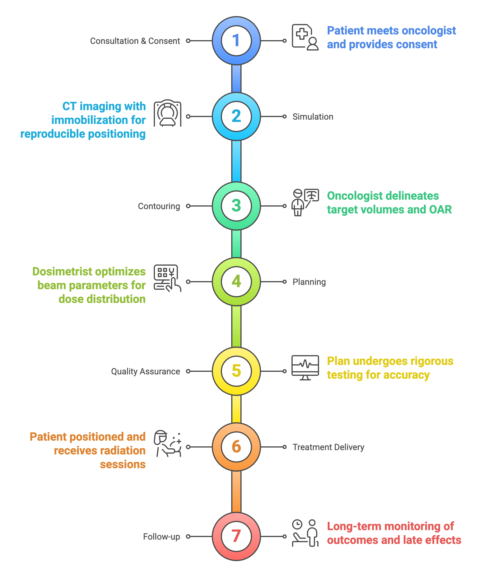
The seven stages of the RT workflow. Figure generated using napkin.ai

The RT workflow, includes seven key stages designed to ensure safe and effective treatment. After initial consultation and consent, the process begins with simulation, where a planning Computed Tomography (CT) volume is acquired using immobilization devices to maintain consistent positioning [Dyer et al., 2019]. While CT is the standard for planning, additional imaging such as Magnetic Resonance Imaging (MRI) or Positron Emission Tomography (PET) may be registered with the planning CT to improve target definition [Mittauer et al., 2019]. Next is contouring, where radiation oncologists outline the Target Volume (TV) and Organ at Risk (OAR) [Yakar and Etiz, 2021]. In the planning phase, dosimetrists or physicists define beam parameters such as energy, intensity, and angle, using Multi Criteria Optimization (MCO) to maximize tumour coverage while sparing healthy tissue [Hussein et al., 2018]. The plan then undergoes QA to confirm its accuracy and adaptability to anatomical changes [Pastor-Serrano and Perk'o, 2021]. Treatment is delivered in multiple sessions, with image guidance used to align the patient before each fraction [Mittauer et al., 2019]. The workflow ends with patient discharge and long-term follow-up to monitor outcomes and late effects [Müller-Polyzou et al., 2024].The entire process from simulation to first treatment can take several days to weeks [Dyer et al., 2019] depending on the complexity of treatment, pointing to the need for more efficient workflows. Each step in the process is elaborated upon next.

Steps in Current Workflow

Patient Consult: The RT workflow starts with a consultation, where the radiation oncologist reviews diagnostic scans, prescribes the dose and fractionation (how many sittings is the treatment delivered in; typically 30 fractions of 2 Gy each for Glioblastoma Multiforme (GBM), with a cumulative prescription of 60 Gy to the TV), and discusses treatment options with the patient [Mittauer et al., 2019, Schiff et al., 2022]. Following this, the patient is scheduled for a CT simulation, the first technical step in planning [Miranda and Miranda, 2021]. Prior to imaging, MRI-safety screening is performed if MRI is part of planning [Moore-Palhares et al., 2023]. Depending on tumour location, immobilization devices may be prepared, such as head and neck masks made in the mould room [Miranda and Miranda, 2021]. Setup instructions and dose details are recorded in the medical record [Moore-Palhares et al., 2023]. Modern workflows increasingly adopt shorter treatment regimens, such as hypo- and single-fractionation, to enhance comfort and reduce visits [Künzel and Thorwarth, 2022].

Imaging and Simulation: The imaging and simulation stage forms the basis of RT planning, with the so-called planning CT as the primary modality for capturing anatomical detail and setup localization [Mittauer et al., 2019]. CT provides tissue density in Hounsfield Units (HU), essential for dose calculation. Additional imaging, such as MRI for soft tissue contrast and PET for metabolic data, enhances target delineation [Pereira et al., 2014]. In advanced workflows like MRI-guided RT, both CT and MRI are acquired and co-registered, with alignment verified by clinical staff [Votta et al., 2024]. Simulation is managed through electronic orders linking treatment systems, imaging devices, and the Treatment Planning System (TPS) [Mori et al., 2012]. The resulting images are used for contouring TV and OAR, establishing patient setup, and calculating radiation dose [Pastor-Serrano and Perk'o, 2021].

Contouring and Target Definitions: After imaging and simulation, the contouring phase is one of the most important steps in the RT workflow. In this step, radiation oncologists outline the target volumes, such as the Gross Tumour Volume (GTV), and identify nearby OARs to spare during treatment [Aselmaa et al., 2017]. Contouring is usually done by drawing 2D outlines on each relevant image slice. These 2D outlines together form the 3D volumes needed for treatment planning [Aselmaa et al., 2017]. Contouring guidelines are used to help outline the TV and OARs correctly. These guidelines improve treatment accuracy and reduce the risk of toxicity [Bentzen et al., 2010]. Different guidelines exist for different parts of the body, which help keep results consistent across clinics. For example, the European Society for RadioTherapy and Oncology (ESTRO)-EANO guideline gives clear advice for contouring in cases of GBM, and recommends using imaging such as MRI to better define the tumour and nearby OARs [Niyazi et al., 2023]. These guidelines help radiation oncologists create high-quality treatment plans across different hospitals [DAHANCA et al., 2015].

Modern RT often uses automatic contouring tools to save time and reduce variation. Systems like Radiation Planning Assistant (RPA) can draw outlines for normal tissues and some target volumes. Radiation oncologists then check and edit these outlines before drawing the GTV themselves [Court et al., 2023, Court et al., 2018]. This method is useful for precise planning, where the automatic contours may still need some editing [Court et al., 2024].

Treatment Planning: After contouring, the outlined TV and OAR are used in the next step called treatment planning. The Clinical Target Volume (CTV) is drawn by expanding the GTV to account for microscopic extensions. The Planning Target Volume (PTV) is then created by expanding the CTV, while avoiding overlaps with OARs. Dose prescriptions and goals for OAR are also set at this stage [Aliotta et al., 2020]. The dose is measured in Gray (equal to 100 rad), which measures one joule of radiation energy absorbed per kilogram of tissue. This contour data is sent from the contouring software to the TPS, where the resulting images are used to calculate radiation dose [Chaves-de-Plaza et al., 2022, Siebert et al., 2022]. This step is critical because it converts anatomical information into a plan that can be used for delivering radiation. Planning starts with treatment setup, which includes defining the isocenter, choosing the beam arrangement, and setting the dose prescription [Gao et al., 2024]. In conventional external beam therapy, beams are usually placed to intersect at the isocenter, which is often the centre of the tumour. Parameters such as beam weights, wedge filters, and Multi-Leaf Collimator (MLC) positions are also defined at this stage [Fernandes et al., 2018].

The planning method depends on the complexity of the treatment. For simpler plans, such as three-dimensional conformal RT, forward planning is used. In this approach, clinicians can manually adjust beam settings to achieve an acceptable dose distribution [Fernandes et al., 2018]. For more complex techniques like Intensity-Modulated Radiotherapy (IMRT) or Volumetric Modulated Arc Therapy (VMAT), inverse planning is required, where the specialized TPS calculates beam settings based on dose constraints provided by the physician [Wang et al., 2020]. They create custom treatment plans that deliver the prescribed dose to the outlined target volumes [Munbodh et al., 2022]. In many centres, staff rotate planning responsibilities. Most plans are completed within two to four days [Siebert et al., 2022].

IMRT uses computer-controlled linear accelerators to adjust beam intensity across many small segments, known as beamlets. This allows for precise dose delivery that fits the shape of the tumour [Cho, 2018]. Inverse planning software is used to define the desired dose, and the system then finds the best beam intensities to meet these goals [Ezzell et al., 2003]. MLCs help shape the radiation beam to match the tumour’s outline during treatment [LoSasso, 2008]. IMRT is especially useful for tumours close to sensitive structures, such as those in the head and neck, prostate, or brain. It helps reduce side effects and improve tumour control [Nutting et al., 2011]. The precision of IMRT also makes it possible to increase the dose to the tumour while protecting nearby healthy tissue [Zelefsky et al., 2002].

VMAT is another advanced technique, which delivers radiation while the machine rotates around the patient. The beam intensity and shape change continuously during the rotation [Otto, 2008]. This method provides a highly conformal dose distribution, and can improve tumour coverage and offer higher protection to nearby normal tissues [Quan et al., 2012]. Compared to IMRT, VMAT can reduce treatment time and the number of Monitor Unit (MU) used, which improves patient comfort and clinic workflow [Palma et al., 2008].

New planning methods also use knowledge-based tools. For example, RapidPlanTM (by Varian, a Siemens Healthineers Company. From: https://www.varian.com/products/radiotherapy/treatment-planning/rapidplan-knowledge-based-planning.) can predict the expected Dose-Volume Histogram before final adjustments are made [Callens et al., 2024]. The Dose-Volume Histogram (DVH) is a chart that shows how radiation dose is spread within different volumes. Another tool is the isodose line map, which connects points that receive the same dose using coloured lines. Systems like the RPA can create complete treatment plans with very little manual input for certain types of cancers [Court et al., 2023, Court et al., 2018]. After optimization, the TPS calculates the dose distribution, using models such as the Anisotropic Analytical Algorithm (AAA) or Acuros XB [Callens et al., 2024]. The grid size for dose calculation is important. A spacing of 2.5 mm is often used because it keeps the dose error below one percent [Callens et al., 2024, Dempsey et al., 2005].

Once the plan is complete, its quality is checked against the clinical goals. If the plan does not meet the goals, parameters are adjusted and the optimization is repeated [Gao et al., 2024]. In automated systems, this cycle continues in the background until the plan meets the required standards [Gao et al., 2024]. The final result is a treatment plan that delivers the prescribed dose to the tumour while protecting OARs, becoming the basis for delivering RT. Treatment planning requires advanced skills and is often the most complex and time-consuming part of the RT workflow [Aliotta et al., 2020, Bellotti et al., 2024].

Plan Review and QA: After treatment planning, all RT plans go through the critical QA phase. This step checks the safety, accuracy, and deliverability of the plan [Munbodh et al., 2022]. Key metrics include the Conformity Index (CI), which shows how well the dose matches the target shape, and the Homogeneity Index (HI), which measures how evenly the dose is spread. Other metrics include the dose to 95% of the target, mean dose, and how much of an organ receives a set dose.

The first review is done by the medical physicist who created the plan, and a second check is done by another qualified physicist who was not involved in the original planning [Iijima et al., 2024]. Some centres also use automated plan-checking software. After the physics review/s, a radiation oncologist reviews the plan to confirm it matches the treatment intent [Siebert et al., 2022].

For complex techniques like IMRT and VMAT, extra checks are done to confirm the machine can deliver the planned dose accurately [Yuan et al., 2018]. This is usually done on the same day as the first treatment. The plan is delivered to a phantom, and the measured dose is compared to the calculated dose. Many centres also review plans in group meetings where doctors and physicists give feedback [Munbodh et al., 2022]. This team-based review adds another layer of safety and ensures consistent treatment quality.

Studies have shown that human review is still essential, even in automated systems [Court et al., 2024, Nealon et al., 2023]. The QA process involves several professionals, each checking different parts of the plan [Siebert et al., 2022]. Clear communication between team members is important to avoid delays or mistakes [Yan et al., 2024]. Rushed reviews to meet deadlines can increase errors, so enough time must be given for proper checks [Yan et al., 2024].

After all reviews and approvals, the plan is sent from the TPS to the electronic medical record [Mittauer et al., 2019, Munbodh et al., 2022]. The plan is then ready for treatment delivery, marking the end of the planning and QA process [Chowdhry and Simpson, 2022].

Treatment Delivery: After plan approval and QA, the patient enters the treatment delivery phase. At each session, radiation therapists position the patient using immobilization devices from simulation [Mittauer et al., 2019]. Image-guided RT, often using volumetric imaging such as Cone-Beam Computed Tomography (CBCT), is performed to verify patient and target alignment with the simulation reference [Schiff et al., 2022]. The workflow follows a strict sequence to ensure treatment matches the approved plan and maintains safety [Chowdhry and Simpson, 2022]. Once alignment is confirmed, radiation is delivered, typically with photon beams of prescribed energy, coordinated through a treatment management system that tracks each step [Mori et al., 2012].

Advanced techniques may be used in complex cases. In online adaptive RT, real-time adjustments are made based on updated imaging, often using MRI, with auto-contouring and dose recalculation based on current anatomy [Lamb et al., 2017]. For mobile targets like in the lung, respiratory gating aligns delivery with specific breathing phases. After treatment, verification may be performed to confirm accurate delivery [Schiff et al., 2022].

Challenges in Contour QA

The manual contour QA process is known to be resource- and time-intensive. It requires strong anatomical knowledge, significant time, and financial support. Manual QA is also subject to inter-observer variability [Loo et al., 2012]. Most errors occur during planning, making pre-treatment contour review essential [Baroudi et al., 2023]. Time constraints are a major challenge, as evidenced by a survey which found that 58% of respondents cited limited time, and 22% cited lack of access to disease site experts, as barriers to effective contour review [Zhang et al., 2021]. These challenges are worse in adaptive RT, where reviewing auto-contours increases clinician workload and reduces patient comfort [Chen et al., 2020]. Automated systems that flag poor-quality contours for manual review can improve efficiency in such cases [Chen et al., 2020].

The quality of RT directly affects treatment outcomes, especially in clinical trials. Many trial centres do not fully review contours after initial checks [Nijhuis et al., 2021]. Poor-quality RT can lead to lower survival and more treatment failures [Zhong et al., 2019]. A major trial in head and neck cancer showed worse outcomes in patients with protocol violations. Two-year survival was 50% vs 70%, and local control was 54% vs 78%, for non-compliant vs compliant plans, respectively [Peters et al., 2010]. Studies also report contouring errors during pre-trial QA in lung cancer trials [Tsang et al., 2019]. Benchmark assessments help identify protocol misinterpretations. These can be addressed by QA teams and trial coordinators [Gwynne et al., 2013, Tsang et al., 2015, Tsang et al., 2019].

The integration of contour QA into clinical practice remains uneven. It is more common in academic centres and institutions with more staff, reflecting resource gaps [Zhang et al., 2021]. Automated contour QA requires checks for each case and for system-wide changes like imaging updates [Jin et al., 2023]. Risk analysis studies using failure mode and effects analysis show that human error remains a key risk in automated workflows. This supports the continued need for manual review by clinicians and physicists [Kisling et al., 2019].

Studies show that contour quality is strongly linked to institutional experience. Centres treating fewer than five patients had a 29.8% rate of major contour issues, compared to 5.4% in centres treating 20 or more patients (p<0.001) [Dragan et al., 2024, Peters et al., 2010]. This shows that experience and specialization improve contour quality. Poor contours can also affect research. Errors in contour data can distort machine learning models used to predict treatment outcomes [Shah et al., 2018]. Contour QA is therefore essential for both patient care and data reliability in treatment development.

An Artificial Intelligence (AI) Primer

Artificial Intelligence (AI) has a large impact on the field of radiation oncology by supporting the entire treatment workflow, from diagnosis to post-treatment care [Fionda et al., 2020, Osman, 2019]. Applications include image contouring, treatment planning, outcome prediction, QA, and adaptive re-planning [Kiser et al., 2019]. AI tools often perform at the level of human experts but in much less time [Kawamura et al., 2023] and can help meet rising demand for RT and support more equal access to care [Nardone et al., 2024].

The modern field of AI has its roots in the 1950s, though related ideas existed earlier. The 1956 Dartmouth Conference is seen as the start of AI, where researchers like McCarthy and Minsky discussed creating what they called “thinking machines” [McCarthy et al., 2006]. More modestly, machine learning aims developing algorithms that can learn patterns from data without being explicitly programmed [Mitchell, 2006]. Early progress was followed by setbacks known as “AI winters,” when funding and results slowed [Toosi et al., 2021]. Early systems were rule-based to model human knowledge but struggled with real-world problems [Dreyfus, 1968, Russell and Norvig, 2016]. AI has advanced through several key shifts from rule-based systems in the 1970s–80s, evolving to statistical models in the 1990s [Dhar, 2024]. The current wave began around 2012 with DL and major improvements in image recognition [Krizhevsky et al., 2012]. This progress is reflected in radiation oncology, which also moved from rule-based tools to statistical models, and now to Deep Learning (DL)-based systems for image analysis and treatment planning [Huynh et al., 2020].

Learning From Data

The field of AI is typically divided into several learning paradigms, as shown in Figure..

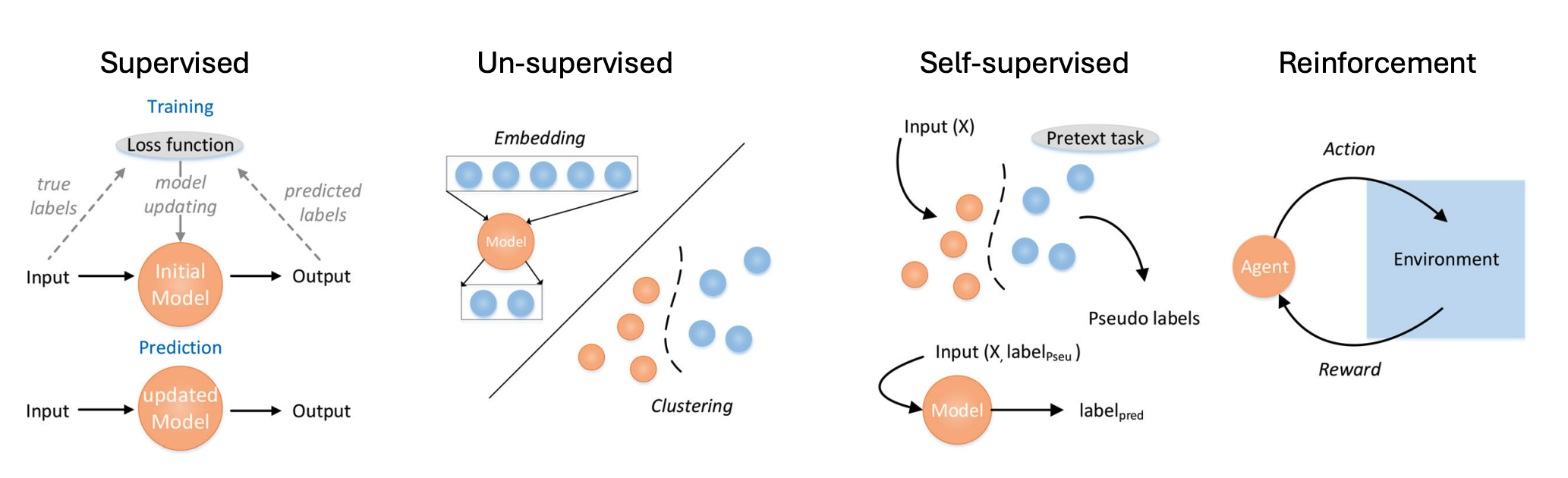
Categories of machine learning, adapted from [Liu and Wu, 2023]: Supervised learning: training process is shown above and prediction process is shown below. Unsupervised learning: the main two applications, embedding and clustering. Reinforcement learning: learn from environment and update from feedback. Self-supervised learning: a pretext task in self-supervised learning is a task designed to train a neural network to learn useful representations of input data without explicit supervision. The network is trained to solve the pretext task using the input data as the only source of supervision, and the learned representations can be transferred to downstream tasks where explicit supervision is available.

Supervised Learning uses labelled data to train models. Each input has a known output, and the model learns to match inputs to outputs by reducing the error between its predictions and the true labels [Russell and Norvig, 2016]. This method is useful in radiation oncology for tasks like tumour classification, where past cases with confirmed diagnoses can be used for training. The success of supervised learning depends on both the quality and quantity of the labelled data. In medicine, creating these labels often needs expert input, which takes time and can be costly. In radiation oncology, inter-expert variability in tasks like contouring can lead to inconsistent training data [Huynh et al., 2020]. Common tasks include classification (e.g., identifying cancerous tissue) and regression (e.g., predicting radiation dose) [Luo et al., 2020].

Unsupervised Learning works with unlabelled data. It finds patterns or groups in the data without knowing the correct outputs [Kohonen, 1990]. One main method is clustering, where similar data points are grouped based on distance or similarity. In radiation oncology, clustering can help identify patient groups with similar treatment responses or uncover trends in treatment plans [Xu and Wunsch, 2005]. Dimensionality reduction techniques like Principal Components Analysis (PCA) and t-SNE [Van der Maaten and Hinton, 2008] help simplify complex data and make it easier to understand. These are useful for visualizing the high-dimensional data common in radiation planning. Unsupervised methods can also detect outliers, which may indicate rare anatomy, equipment errors, or issues in treatment plans [Huang et al., 2023].

Semi- or Self-Supervised Learning (SSL) combine supervised and unsupervised methods by using a small amount of labelled data and a larger set of unlabelled data. This is helpful in medical imaging, where unlabelled scans are common but expert annotations are limited [Cheplygina et al., 2019]. In self-supervised learning, the model creates its own learning tasks using unlabelled data. For example, it may learn to predict missing parts of an image using the full image as a reference [Chen et al., 2019]. SSL frameworks such as SimCLR [Chen et al., 2020], DIstillation with NO labels (DINO) [Caron et al., 2021], and masked auto-encoders [He et al., 2022] are used to pre-train models, which can help with tasks like contouring. Other models like Mean Teacher [Tarvainen and Valpola, 2017] and FixMatch [Sohn et al., 2020] use pseudo-labelling and consistency regularization, which are important when only a few labelled samples are available.

Reinforcement Learning teaches models to make decisions by using rewards. There are no labelled outputs. Instead, the model learns from trial and error by receiving rewards for good actions and penalties for bad ones.

Limitations of Traditional Machine Learning: While traditional machine learning algorithms have proven valuable in many applications, they have several limitations that DL addresses:

• Feature engineering dependency: Traditional algorithms rely heavily on manual feature engineering, which requires domain expertise and can miss complex patterns that aren’t explicitly encoded [Jiang et al., 2018].

• Difficulty with unstructured data: Images, text, and other unstructured data types are challenging for traditional algorithms without extensive preprocessing [Shen et al., 2017].

• Limited representation capacity: Many traditional algorithms struggle to capture complex, hierarchical patterns in data [Bengio et al., 2013].

• Fixed model complexity: The complexity of traditional models is often fixed or limited by design, constraining their ability to scale with data size [Goodfellow et al., 2016].

• Separate learning stages: Traditional pipelines often involve separate stages for feature extraction and model training, preventing end-to-end optimization [LeCun et al., 2015].

DL addresses these limitations through its ability to automatically learn hierarchical representations from raw data, scale with data and computational resources, and enable end-to-end training [LeCun et al., 2015]. However, traditional methods retain advantages in scenarios with limited data, when interpretability is crucial, or when computational resources are constrained [Rudin, 2019].

Evolution of DL for Computer Vision

DL refers to a group of machine learning models inspired by how the human brain works [LeCun et al., 2015]. These models use many layers of connected units, called artificial neurons, to process and learn from data [Schmidhuber, 2015]. The term “deep” comes from the presence of multiple hidden layers between the input and output [Goodfellow et al., 2016].

Each artificial neuron receives inputs, multiplies them by weights, applies a non-linear function, and produces an output. When combined in layers and trained on large datasets, these neurons can detect patterns and make predictions. The layered structure allows the model to learn features at different levels of complexity, reducing the need for manual feature design [Bengio et al., 2013].

DL has driven major progress in AI since the early 2010s [Jordan and Mitchell, 2015]. This progress is due to larger datasets, better computing power (especially from Graphics Processing Unit (GPU)s), and improvements in training methods [Schmidhuber, 2015].

Theoretical Foundations: DL is effective because of two key capabilities: performing region-wise computations with non-linear transformations over large receptive fields, and using efficient gradient-descent training through back-propagation [Ionescu et al., 2015]. These strengths have allowed DL to outperform older models that relied on hand-crafted features.

The Convolutional Neural Network (CNN) is the most widely used deep learning model for visual tasks. Developed in the late 1980s by Yann LeCun, CNNs are designed to learn spatial patterns in grid-based data such as images [Mohimont et al., 2022]. They use convolution filters that scan across the image, sharing weights to reduce the number of parameters and improve efficiency [Gojić et al., 2022]. A typical CNN has several layers stacked together to extract spatial features. During training, the model adjusts its parameters to reduce the difference between its predictions and the ground truth [Gojić et al., 2022], which allows CNNs to learn features directly from the data, removing the need for manual feature engineering [Ali et al., 2020]. Feature learning in DL is hierarchical, where early layers learn basic patterns like edges or colours, while deeper layers capture more specific and complex features [Zeiler and Fergus, 2013]. This makes transfer learning possible, where models trained on large datasets can be adapted to new tasks with less data [Mohimont et al., 2022].

Modern DL models often use a modular design. A “backbone” network extracts general features, and a “head” network performs a specific task such as classification or segmentation [Ali et al., 2020]. This design supports the development of task-specific architectures like U-Net, which is widely used for biomedical image segmentation [Ronneberger et al., 2015]. When trained on enough data, these models can generalize well and achieve strong performance on tasks like classification and segmentation [Littek et al., 2023].

Architectural Innovations: The development of DL architectures has transformed computer vision, evolving from general classifiers to specialized segmentation models. Before this shift, segmentation relied on edge- or region-based methods [Xiong et al., 2020]. Early CNNs like AlexNet, VGG-16, GoogLeNet, and ResNet introduced key components later reused in segmentation networks [He et al., 2015, Krizhevsky et al., 2012, Szegedy et al., 2014]. A major breakthrough came with Fully Convolutional Network (FCN), which enabled end-to-end pixel-level predictions by removing fully connected layers [Shelhamer et al., 2014]. This approach adapted classification networks for segmentation through fine-tuning and influenced many later methods [Polewski et al., 2024].

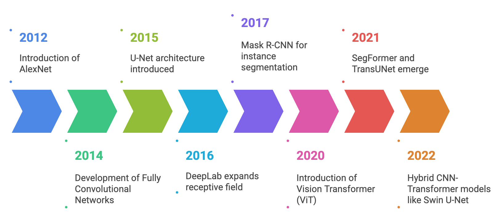
Evolution of DL architectures for image segmentation: from FCNs to transformer based models and multi-modal architectures. Figure generated using napkin.ai

Encoder-decoder architectures, such as U-Net and SegNet, became widely used for their ability to combine contextual understanding with precise localization [Badrinarayanan et al., 2015]. U-Net, in particular, proved effective in medical imaging with limited data [Ronneberger et al., 2015]. Dilated convolution networks like DeepLab expanded the receptive field without increasing parameters and introduced techniques such as Atrous Spatial Pyramid Pooling (ASPP) and Continuous Random Field (CRF)s for better boundary detection [Chen et al., 2016]. Other models, including deconvolution networks and large-kernel approaches, further improved segmentation detail and performance [Noh et al., 2015, Peng et al., 2017]. Instance segmentation progressed through top-down methods like Mask R-CNN [He et al., 2017] and bottom-up approaches like Deep Watershed Transform [Bai and Urtasun, 2016].

Attention mechanisms improved global context modelling. Architectures such as Attention Gated U-Net (AGU-Net) enhanced U-Net by highlighting important regions, aiding detection of small or subtle structures [Schlemper et al., 2019]. Transformers, introduced through Vision Transformer (ViT) [Dosovitskiy et al., 2020], were later adapted for segmentation with models like SegFormer, TransUNet, and U-Net + Transformer Hybrid (UNETR), offering strong performance in complex medical tasks [Chen et al., 2021, Hatamizadeh et al., 2022, Xie et al., 2021]. Hybrid CNN-Transformer models, including Swin U-Net and CoTr, combined local feature extraction with global attention, proving effective for 3D data [Cao et al., 2022, Li et al., 2022]. 3D and multimodal fusion architectures like nnU-Net and V-Net are now standard in volumetric segmentation tasks using MRI and CT, often incorporating multi-modal inputs for better accuracy [Isensee et al., 2021, Milletarì et al., 2016].

Modern segmentation models deliver high accuracy and efficiency, turning segmentation into a robust, end-to-end process with wide applications [Alokasi and Ahmad, 2022].

U-Net Architecture: U-Net, introduced by Ronneberger et al. in 2015, is a widely used architecture for semantic segmentation, especially in medical imaging [Ronneberger et al., 2015]. It features a symmetric encoder-decoder design, with skip connections that link encoder and decoder layers to retain spatial details lost during downsampling. These connections also help with gradient flow and improve training stability [Zhou et al., 2018]. Originally developed for biomedical images, U-Net showed strong performance with limited training data, aided by extensive data augmentation. It is efficient, segmenting high-resolution images in under a second on modern GPUs [Ronneberger et al., 2015], and has become a standard in many domains [Zhang et al., 2021].

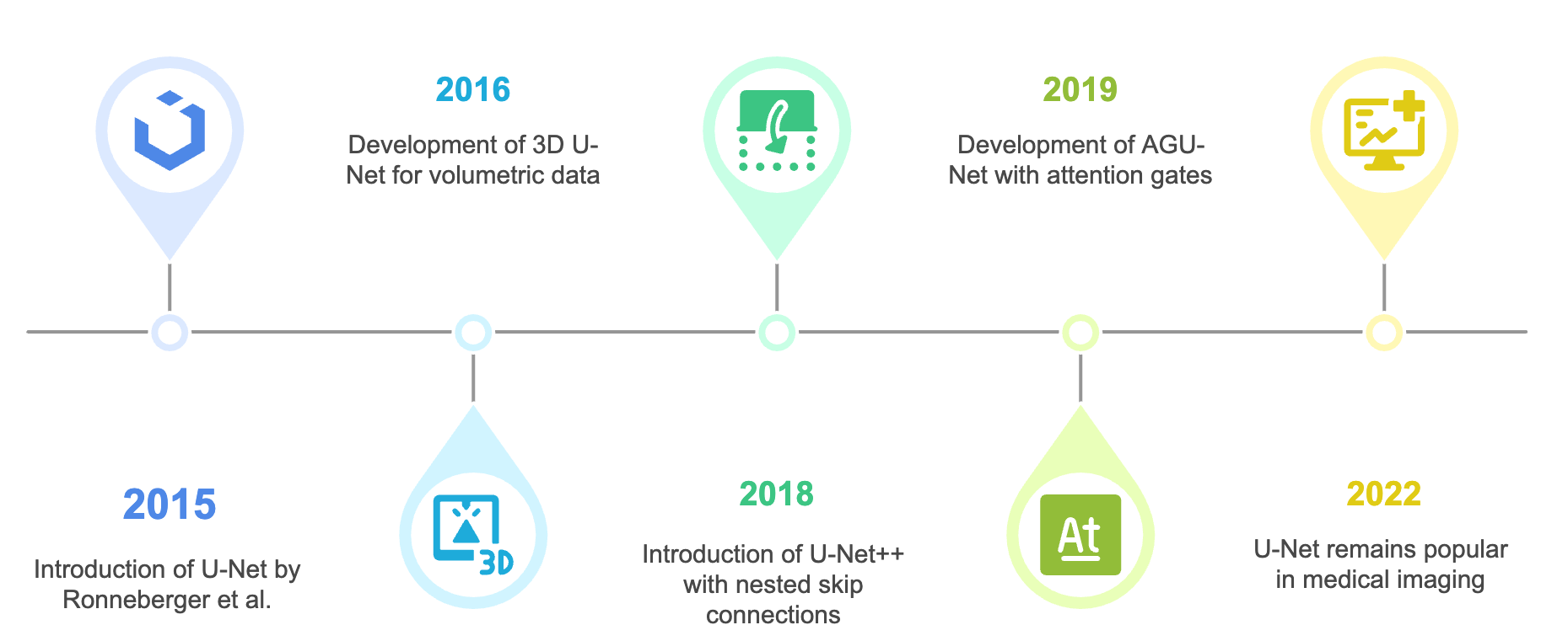
The U-Net architecture has evolved several variations based on backbone, skip-connection, and data-flow enhancements. Figure generated using napkin.ai

3D U-Net extends this approach to volumetric data by using 3D operations and online elastic deformations for augmentation [Çiçek et al., 2016]. Variants like U-Net with multiple skip-connections (UNet++) improve feature alignment between encoder and decoder paths using nested skip connections [Zhou et al., 2018]. U-Net has also been adapted to use different encoder backbones, such as ResNet, to leverage transfer learning [Ali et al., 2025]. Lightweight versions reduce computation by using fewer layers and simpler upsampling, though often at the cost of detail around object boundaries [Liu and Yin, 2019].

The evolution of U-Nets across the past decade has been. Further developments include AGU-Net, which uses attention gates to focus on important regions [Schlemper et al., 2019], and V-Net, which uses a Dice Similarity Coefficient (DSC)-based loss to address class imbalance in 3D segmentation [Milletarì et al., 2016]. U-Net remains popular due to its balance of accuracy, speed, and adaptability. Its success with small datasets makes it ideal for medical imaging, and it continues to serve as the foundation for newer segmentation architectures [Azad et al., 2022].

Related Work

AI in Contouring

In recent years, AI, and particularly DL, has significantly advanced auto-contouring in radiation therapy (RT). These approaches have consistently outperformed conventional atlas-based methods [Radici et al., 2022]. A notable milestone was the 2017 American Association of Physicists in Medicine (AAPM) Grand Challenge, where DL models surpassed the previous gold standard model-based methods for thoracic anatomy segmentation on CT scans [Roper et al., 2022, Yang et al., 2018]. Other studies have similarly shown that DL-based segmentation yields more accurate results than atlas-based techniques [Bustos et al., 2023, Radici et al., 2022]. While atlas-based methods rely on registering annotated CT datasets to new patient scans, DL models use CNNs trained to detect spatial patterns and variations of anatomical structures [Bustos et al., 2023]. This shift marks a major advancement in auto-contouring technology [Heilemann et al., 2023].

The implementation of AI-based auto-contouring brings several benefits to clinical practice. It can reduce clinician workload, improve workflow efficiency, and enhance standardization across institutions and users [You et al., 2022]. These advantages are particularly relevant in time-sensitive procedures such as brachytherapy, where implanted needles or applicators increase the complexity of contouring [Kraus et al., 2023]. Moreover, rapid and accurate contour generation supports the development of online adaptive RT [Heilemann et al., 2023]. The commercial landscape for auto-contouring has also expanded, with both established vendors and new companies offering AI-driven solutions [Wang et al., 2025]. This growth is driven by the ongoing need to address challenges in manual contouring, including inter-observer variability, time constraints, and the increasing complexity of modalities such as stereotactic radiosurgery (Stereotactic Radiosurgery (SRS)) and stereotactic body radiotherapy (Stereotactic Body Radiation Therapy (SBRT)) [Bustos et al., 2023].

The accuracy and clinical performance of AI-based auto-contouring tools have been widely evaluated. Studies often report results using quantitative metrics such as the DSC, Mean Surface Distance (MSD), and HD to compare AI-generated contours with those created manually, consistently showing that AI-based tools can match or even exceed expert-level performance.

Evolution of Auto-contouring Systems: The evolution of auto-contouring techniques in radiation therapy has followed several distinct phases, each aimed at overcoming the limitations of earlier methods. Initial efforts relied on simple techniques such as image value thresholding to automate segmentation tasks [Radici et al., 2022]. These early approaches were eventually replaced by more advanced atlas-based auto-segmentation (Atlas-Based Auto-Segmentation (ABAS)) methods, which became widely used in clinical practice over the past decade [Vrtovec et al., 2020].

A major shift occurred with the introduction of AI, particularly DL methods. DL algorithms, based on CNNs, are trained to identify spatial features and anatomical variations in medical images [Bustos et al., 2023]. This transition from atlas-based to DL-based auto-contouring has accelerated in recent years, supported by rapid advancements in algorithm development and increasing clinical adoption of AI-based segmentation tools [Wang et al., 2025].

Over the past several decades, various methodologies have been developed for auto-contouring in RT, including the following:

Atlas-Based Segmentation: This method involves registering previously contoured CT datasets to new patient scans and transferring contours accordingly. Although atlas-based approaches represented a significant advancement over manual contouring, they are limited by their sensitivity to differences in image quality between reference and target CT scans, as well as by the accuracy of registration algorithms and the effectiveness of post-processing steps [Bustos et al., 2023]. These systems typically require substantial computational resources and several minutes per case. Despite widespread adoption, optimal atlas selection remains a challenge, with evidence suggesting that even state-of-the-art selection algorithms perform suboptimally compared to ideal selection benchmarks [Schipaanboord et al., 2019].

Machine Learning Approaches: These approaches leverage algorithms capable of detecting patterns through learning processes, enabling more adaptable integration of prior knowledge for anatomical structure labelling [Boon et al., 2018, Hu et al., 2023]. While the majority of prior research has focused on improving model architecture with fixed datasets (a model-centric approach), recent interest has shifted toward data-centric strategies, where the focus is on enhancing data quality while using fixed models [Hamid, 2022, Wahid et al., 2023].

DL: has become the most widely used framework for medical image segmentation. Architectures such as U-Net have gained popularity due to their ability to balance global context with precise spatial localization, while also performing well with limited training data [Ronneberger et al., 2015]. Similarly, 3D U-Net architectures [Çiçek et al., 2016] have demonstrated strong generalization across international datasets for head and neck OAR segmentation, performing comparably to expert clinicians [Nikolov et al., 2018]. More recently, ViT-based models [Hatamizadeh et al., 2022] have been competing against traditional CNNs [Isensee et al., 2021], with various research articles comparing the two [Wald et al., 2025], while Segment Anything Model (SAM)-based models have been modified for medical imaging workflows to demonstrate significant time-savings in the auto-contouring process [Isensee et al., 2025].

Deep Learning for GBM Target Delineation: Auto-segmentation of glioblastoma (GBM) target volumes has the potential to significantly reduce inter-observer variability and accelerate the planning process. While most previous DL-based methods have focused on pre-operative tumour segmentation without incorporating surrounding OARs or post-surgical cavities [Bakas et al., 2018, Kickingereder et al., 2019, Menze et al., 2014], recent models have been developed to address these limitations [Sadeghi et al., 2023]. Comparative studies consistently report that DL-based approaches outperform atlas-based methods in target delineation accuracy across various anatomical regions [Li et al., 2022, Ng et al., 2022, Wang et al., 2022]. For example, combining deep learning-based auto-contouring with manual corrections has been shown to improve accuracy and efficiency in post-operative lung cancer CTV delineation [Bi et al., 2019], although no equivalent studies currently exist for GBM.

Commercial Implementations: The transition to AI-driven segmentation has led to rapid commercial development. Numerous vendors now offer pre-trained, clinically deployable auto-contouring tools [Heilemann et al., 2023, Wang et al., 2025]. These include products from Manteia Medical Technologies, Mirada Medical, and Carina Medical, among others [Chen et al., 2020, Ng et al., 2022]. Such solutions have demonstrated measurable benefits in improving the efficiency of OAR segmentation and reducing inter-observer variability across clinical workflows [Wang et al., 2025].

Anatomical Sites: Comparative studies across multiple anatomical regions using seven different AI systems show that no single platform consistently performs best across all sites, highlighting the need to tailor tool selection to specific clinical contexts [Choi et al., 2024, Kim et al., 2024, Meyer et al., 2024]. Anatomy-specific models have shown strong performance in various cancer types.

In head and neck cancer, 3D U-Net architectures generalize well across international datasets, achieving expert-level accuracy. Clinical adoption is growing, with up to 50% of auto-contours used without modification and time savings of up to 112 minutes per case [Boon et al., 2018]. For glioblastoma, CNN-based segmentation has addressed the variability and effort of manual contouring [Sadeghi et al., 2023]. In nasopharyngeal cancer, AI tools achieved 79% accuracy and reduced both inter-observer variability (by 54.5%) and contouring time (by 39.4%) [Chen et al., 2021, Lin et al., 2019].

DL models in breast cancer significantly reduce contouring time, in some cases from 40 to 10 minutes [You et al., 2022]. For lung cancer, DL-assisted methods improve segmentation accuracy and reduce planning time by 35%, with multi-centre trials reporting reduced inter-observer variability by about 50% [Bi et al., 2019, Chen et al., 2021, Han et al., 2024].

In cervical cancer, VB-Net models achieved DSC up to 0.88, with 63.5% of contours requiring only minor edits. Performance was comparable to senior clinicians and superior to junior ones [Kraus et al., 2023, Ma et al., 2021]. In prostate cancer, 45% of surveyed oncologists already use AI tools clinically, reporting time savings up to 72% [Hindocha et al., 2023, Meyer et al., 2024]. For colorectal cancer, recent studies have demonstrated growing applicability of AI-based methods [Chen et al., 2021, Meyer et al., 2024].

Benefits and Challenges of using AI-contouring: AI-based auto-contouring significantly reduces inter-observer variability. In nasopharyngeal carcinoma, it lowered variation by 54.5% [Chen et al., 2021, Lin et al., 2019], and in lung cancer, variation decreased by approximately 50% [Han et al., 2024]. This consistency supports more standardized RT planning. Efficiency gains are also notable. Time savings range from 35% in lung cancer [Bi et al., 2019, Chen et al., 2021] to 39.4% in nasopharyngeal carcinoma [Chen et al., 2021, Lin et al., 2019], and up to 72% and 84% in prostate and head and neck cancers, respectively [Hoque et al., 2023].

Despite these benefits, contour revisions can be time-consuming. In some cases, correcting AI-generated contours takes nearly as long as manual contouring [Bai et al., 2021], especially in adaptive workflows like proton therapy [Chaves-de-Plaza et al., 2022]. Human oversight remains essential. While AI improves consistency, clinical review ensures accuracy and safety [Hoque et al., 2023]. Implementation also requires adherence to standardized contouring protocols, as clinician-AI discrepancies may affect planning outcomes [Adams et al., 2023]. AI tools often perform inconsistently across anatomical regions. Accuracy drops for small or complex structures, and no single platform outperforms others across all sites [Kim et al., 2024], requiring careful tool selection per clinical context.

The “black box” nature of AI presents challenges. Limited model interpretability and reliance on training data affect clinician trust and integration into clinical practice [Heilemann et al., 2023]. User training also influences outcomes. Less experienced users may spend more time adjusting contours, underscoring the need for proper training [Goddard et al., 2024, Zhong et al., 2021]. Effective clinical use depends on strong QA protocols. Human review is still essential to ensure reliability and mitigate errors [Hoque et al., 2023]. Model performance depends on the quality and diversity of training data. Lack of representative datasets can limit generalizability to real-world clinical scenarios [Heilemann et al., 2023].

Finally, adaptable models are needed to address diverse 3D structures and imaging modalities [Chen et al., 2024]. While AI tools are not yet perfect, they provide major gains in efficiency and standardization, enhancing modern RT workflows [Shanbhag et al., 2023].

Robust Auto-contour Models

The growing reliance on DL models for contouring and treatment planning makes robustness essential for building trust among clinicians and patients. Reliable performance across anatomical and imaging variations is critical, especially in volumetric models that, despite strong results in organ and tumour segmentation, remain vulnerable to adversarial attacks [Malik et al., 2024, Zou et al., 2023]. Poor RT quality has been linked to treatment failure, lower survival, and increased toxicity in clinical trials [Peters et al., 2010].

In oncology, robust contouring is vital for accurate tumour analysis and planning. Radiomics depends on precise contours to extract imaging biomarkers that guide treatment. Even small contouring errors can impact therapy decisions or lead to missed diagnoses [Wu et al., 2021]. Robust features also help identify tumour subtypes with distinct molecular traits and outcomes [Suter et al., 2020]. The use of multiple imaging modalities such as CT, MRI, and ultrasound further highlights the need for consistent auto-contouring. Models capable of stable performance across modalities support standardized treatment planning across diverse clinical environments. However, even state-of-the-art models like SAM show limitations in multi-modal, multi-object segmentation tasks [Shi et al., 2024].

Necessity for Robustness of State-of-the-art Solutions: The reliability of DL systems depends on both accuracy and robustness to input perturbations. Recent studies suggest that medical image segmentation models may be more vulnerable to adversarial attacks than previously believed, raising concerns for clinical use [Daza et al., 2021]. Sensitivity analysis is crucial in evaluating how input variations affect predictions, offering insights into model reliability in diverse anatomical and imaging scenarios [Kuang et al., 2024, Maleki et al., 2024, You and Reyes, 2022].

Robust contouring models are also vital for building trust between clinicians and patients. Consistent model outputs across imaging conditions and patient anatomy help clinicians feel confident in AI-generated contours [Zou et al., 2023], a key factor for adoption. However, improving robustness typically requires extensive expert annotations, posing challenges for deployment in resource-constrained settings [Greenspan et al., 2016]. Models that achieve robustness with fewer labelled examples are more likely to succeed in real-world clinical workflows [You et al., 2023].

Types of Robustness: Auto-contouring models must exhibit several forms of robustness to be clinically reliable. One key type is domain robustness or generalization, the ability to generalize across data from different scanners, protocols, or institutions [Chen et al., 2021, Hwang and Hwang, 2021]. Texture robustness addresses the sensitivity of DL models to textural bias. Simulating textural noise during training can improve invariance and performance on scans affected by unseen noise, especially in 3D data [Chai et al., 2020]. Image quality robustness ensures stable performance under conditions like blur or noise, which are common in intraoperative or real-time settings where training data is often cleaner [Shi et al., 2024]. Modality robustness is also essential. Even foundation models such as SAM show inconsistent performance across imaging modalities, highlighting the difficulty of achieving zero-shot generalization on multi-modal medical datasets [Shi et al., 2024].

Challenges in Building Robust Models: Despite progress, vulnerabilities in clinical deployment remain a concern, highlighting the need for robust solutions where model failure can have serious consequences [Kuang et al., 2024]. A key challenge is intensity inhomogeneity, where varying pixel intensities within the same tissue lead to inaccurate contours [Almasganj and Fatemizadeh, 2025]. This is worsened by common noise types (e.g., Gaussian, speckle) in medical imaging [Wang and Ma, 2016].

Weak boundaries between structures further complicate segmentation, especially in low-contrast or complex regions, often causing clinically relevant errors [Zhang et al., 2023, Zhang et al., 2024]. Poor-quality annotations in datasets also introduce label noise that limits model performance [Shi and Wu, 2021]. Domain shift is another major barrier. Variability in scanners, protocols, and modalities creates distribution mismatches, and DL models often overfit to texture and style cues that do not generalize well [Chen et al., 2024, Li et al., 2024]. Moreover, adversarial attacks, which are imperceptible perturbations crafted to mislead models, pose serious risks to segmentation models [Laousy et al., 2023]. Such attacks are especially concerning in volumetric applications like OAR and TV contouring, where current defences lack theoretical guarantees [Athalye et al., 2018, Daza et al., 2021, Li et al., 2020].

Current Solution Approaches: To address these challenges, local statistics-based models have been used to mitigate intensity inhomogeneity and noise by leveraging localized image features [Zhao, 2024]. Uncertainty estimation is another strategy to flag low-confidence predictions [Zhang et al., 2023, Zhang et al., 2021, Zou et al., 2022], although models remain well-calibrated at the dataset level but not at the subject level [Jungo and Reyes, 2019]. Simulated perturbations via data augmentation or adversarial training have improved robustness across domains and textures [Santhirasekaram et al., 2022].

For modality robustness, uncertainty-based methods help address boundary ambiguities, including probabilistic contouring frameworks [Shi et al., 2024]. Some foundation models have shown improved domain generalization after fine-tuning [Le, 2023]. Addressing these issues requires robust evaluation practices: assessing performance under varied conditions, validating across diverse patient groups, and documenting assumptions about data inputs that may affect clinical outcomes [Maleki et al., 2024, Mzoughi et al., 2025, Rossolini et al., 2022, Tejani et al., 2023].

AI for Fast Dose Predictions and QA

AI is well-suited for radiation oncology for analysing large datasets to improve treatment planning. In IMRT and VMAT, AI models can predict key variables at each planning stage, either by learning from prior clinical plans or by mimicking human decision-making [Sheng et al., 2021]. Integrating AI into RT workflows helps automate repetitive tasks, reduce costs, and enhance QA and patient care [Fionda et al., 2020]. These tools also support clinicians in delivering efficient, personalized treatment aligned with individual patient needs [Fionda et al., 2024].

AI for Treatment Planning: Treatment planning in radiation therapy is complex and time-intensive, demanding manual expertise. AI offers a promising solution to automate and standardize this process, enhancing both efficiency and consistency [Wang et al., 2019]. AI applications fall into two categories: one predicts optimal DVH, 3D dose distributions, or fluence maps based on prior plans; the other mimics human decision-making during optimization [Sheng et al., 2021]. Both reduce trial-and-error, improving plan quality.

Knowledge-Based Planning (KBP) trains models on curated datasets of clinical plans, enabling automatic generation of high-quality plans while reducing variability due to planner experience [Avanzo et al., 2021, Wang et al., 2024]. DL-based models, especially those using CNNs, can directly predict fluence maps from anatomy in seconds, with performance comparable to clinician plans [Wang et al., 2020]. Recent developments include Large Language Model (LLM)-based agents for planning [Nusrat et al., 2025] and systems that auto-generate large numbers of plans to support AI training [Gao et al., 2025], helping standardize workflows and enhance quality [Weidlich and Weidlich, 2018].

AI has proven effective in complex sites like head and neck. The RPA system from M. D. Anderson Cancer Center automates contouring and planning for multiple cancer types, often matching or exceeding manual plan quality while reducing time [Haddad et al., 2018, Nardone et al., 2024]. For prostate SBRT, AI plans rival manual ones on clinical Linear Particle Accelerator (LINAC)s [Roover et al., 2021], while whole breast plans can be optimized in under 20 seconds [Sheng et al., 2019]. Despite these advances, clinical implementation demands rigorous validation. Concerns about robustness in diverse scenarios remain, and outcomes must be verified by clinical physicists [Hito et al., 2021]. Human oversight remains essential for ensuring plan safety and customization for individual anatomy [Avanzo et al., 2021, Wang and White, 2019].

AI for QA: QA is vital in RT, but traditional processes are time-consuming and prone to uncertainty. AI offers automation and accuracy improvements for both machine-specific and patient-specific QA [Kiser et al., 2019, Osman, 2019]. In patient-specific QA, AI models predict gamma passing rates for IMRT and VMAT using plan complexity metrics, achieving accuracies within 3% of measured values via tree-based models like AdaBoost and XGBoost [Lam et al., 2019, Siciarz et al., 2021]. DL models such as CNNs can also classify dose errors (e.g., MLC, monitor units, setup) from dose maps, outperforming basic gamma analysis by identifying root causes [Kimura et al., 2021, Nyflot et al., 2018, Potter et al., 2020, Wolfs and Verhaegen, 2022]. In proton therapy, where traditional systems lack built-in monitor unit calculations, AI models using Gaussian Process Regression (GPR) and neural networks predict output factors with mean errors under 2% [Grewal et al., 2020, Peng et al., 2022, Sun et al., 2018]. Virtual QA using architectures like UNet++ can predict dose distributions and gamma rates without requiring physical measurements, offering faster alternatives [Chen et al., 2023, Deng et al., 2025, Huang et al., 2021].

Medical physicists validate AI models through comparisons with standard dose calculations and phantom tests [Manson et al., 2023]. This is especially important in adaptive RT, where AI can reduce QA workload during daily replanning [Chan et al., 2020, Lemus et al., 2024]. AI models can monitor machine components like MLCs and imaging systems over time, helping predict failures and reduce downtime [Zhao et al., 2021]. Bayesian network tools have been used for automated plan review [Kalendralis et al., 2023], while AI-based contouring systems now undergo QA checks for both geometric and dosimetric validity before use [Hoque et al., 2023]. Challenges remain, as most studies are retrospective or simulated [de Kerf et al., 2023]. Safe deployment, model maintenance, and workflow adaptation are key issues. AI is poised to improve contouring, registration, and real-time adaptive treatment, including MR-based synthetic CT generation and QA integration [Hagawi et al., 2024, Psoroulas et al., 2025].

Evaluation Metrics

Performance evaluation must be tailored to the specific nature of the predictive task, whether classification, regression, segmentation, or treatment planning, and should be grounded in clinical relevance, particularly the potential implications of false positives and false negatives [Hicks et al., 2022]. In the context of biomedical imaging and radiation oncology, a comprehensive set of evaluation metrics is essential for reliable model validation and clinical translation. This section provides an overview of the classification, segmentation and radiation oncology-specific metrics used in the research works that follow.

Classification Tasks

For classification tasks, the following metrics are commonly used:

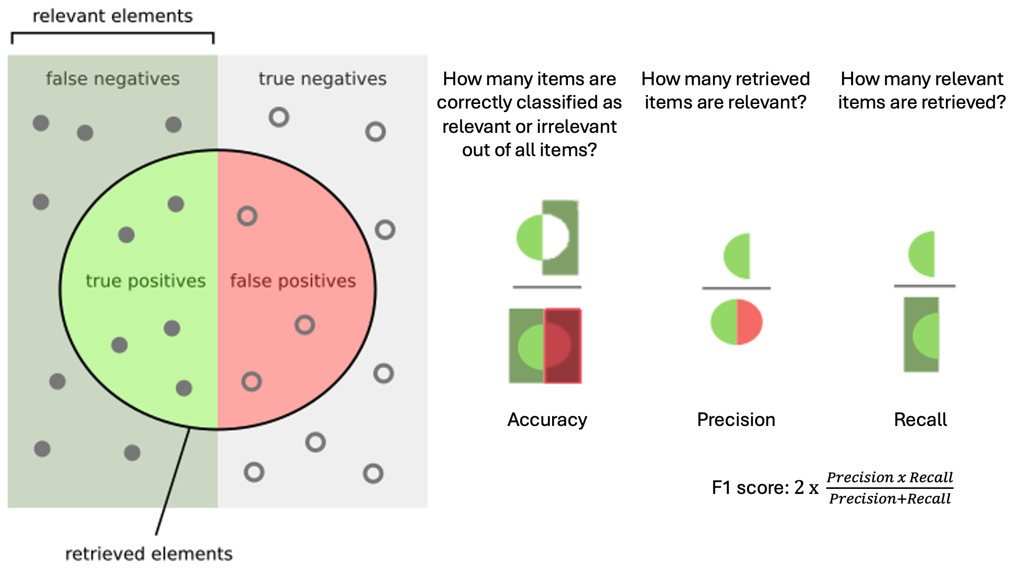
Visualization of typical classification metrics in a binary scenario. Figure adapted and modified from Wikipedia.

• Accuracy:

\[ \text{Accuracy} = \frac{TP + TN}{TP + FP + TN + FN} \]

This represents the proportion of correctly classified instances (true positives and true negatives) out of all predictions. It is most informative in datasets with balanced class distributions but can be misleading in imbalanced datasets, which are common in medical imaging.

• Precision (Positive Predictive Value):

\[ \text{Precision} = \frac{TP}{TP + FP} \]

Precision measures the proportion of predicted positive cases that are actually positive. It is particularly critical when the cost of a false positive is high, such as unnecessary biopsies or treatments.

• Recall (Sensitivity or True Positive Rate):

\[ \text{Recall} = \frac{TP}{TP + FN} \]

Recall captures the ability of the model to correctly identify all actual positive instances. In diagnostic imaging, high sensitivity is often prioritized to minimize the risk of missed detections.

• F1 Score:

\[ \text{F1} = 2 \times \frac{\text{Precision} \times \text{Recall}}{\text{Precision} + \text{Recall}} \]

The F1 score provides a harmonic mean of precision and recall, offering a balanced measure when both false positives and false negatives are clinically consequential.

• Area Under the Receiver Operating Characteristic Curve: The AUC-ROC (Area Under the Receiver Operating Characteristic Curve) quantifies the model’s discriminative capacity across all classification thresholds. It plots the true positive rate against the false positive rate and is particularly useful for comparing classifiers independent of class imbalance [Bradley, 1997].

Segmentation/Contouring Tasks

In segmentation tasks, especially those used in RT for delineating OAR and TV, voxel-wise classification metrics are often insufficient. Instead, spatial agreement metrics are employed to assess the geometric concordance of predicted contours to ground truth annotations [Taha and Hanbury, 2015].

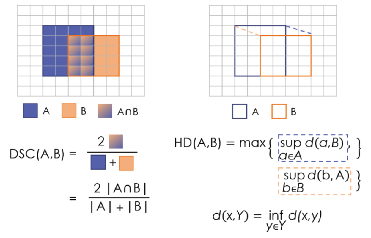
Visualization of the two types of segmentation metrics: overlap based (DSC) and distance based (Hausdorff Distance (HD)). Surface DSC is a variation of DSC only on the borders, and Average Symmetric Surface Distance (ASSD) is a variation of HD. Figure adapted from [Reinke et al., 2021].

• Dice Similarity Coefficient:

\[ \text{DSC} = \frac{2 |\text{A} \cap \text{B}|}{|\text{A}| + |\text{B}|} \]

The DSC [Zou et al., 2004] quantifies volumetric overlap between the predicted segmentation \(A\) and the ground truth \(B\). It ranges from 0 (no overlap) to 1 (perfect overlap) and is widely used for evaluating organ and tumour contours.

• Hausdorff Distance:

\[ \text{HD}(A, B) = \max\left\{\sup_{a \in A} \inf_{b \in B} d(a, b), \sup_{b \in B} \inf_{a \in A} d(b, a)\right\} \]

The HD [Huttenlocher et al., 1993] measures the largest boundary deviation between two contours. It highlights worst-case errors, which are critical in high-precision applications like stereotactic radiotherapy.

• ASSD:

\[ \text{ASSD}(A, B) = \frac{1}{|A| + |B|} \left(\sum_{a \in A} \min_{b \in B} d(a,b) + \sum_{b \in B} \min_{a \in A} d(b,a) \right) \]

ASSD computes the average boundary distance between the predicted and ground truth segmentations, offering a smoother measure than HD and less sensitivity to outliers.

• Surface Dice: A variant of DSC computed on the surface voxels within a tolerance (e.g., 1–2 mm), Surface Dice assesses the fraction of boundary points from one surface that are within a specified distance of the other. This is especially important in clinical settings where small boundary errors can significantly impact dosimetric outcomes [Nikolov et al., 2018].

Radiation Oncology-specific Metrics

In RT, evaluation must extend beyond geometric accuracy to include dose distribution and biological impact. Dose distributions are measured typically using a DVH.

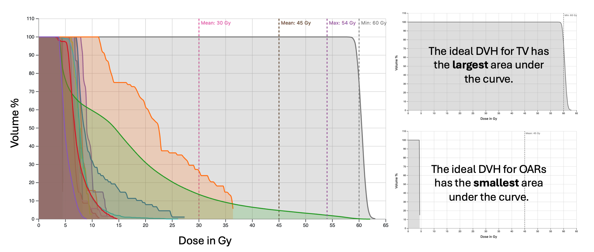
Typical DVH curves: representing 3D doses in a 2D histogram, where percentage of volume receiving levels of doses up to the prescribed treatment dosage is plotted.

It is a two dimensional graph that shows how much radiation dose is received by different volumes of tissue (both tumour TV and OARs). The x-axis represents the radiation dose (in Gray), and the y-axis shows the percentage of the tissue volume receiving at least that dose. By analysing the DVH, clinicians can assess whether a treatment plan is safe and effective. The following domain-specific metrics, some of which are based on points on the DVH plane are used to assess treatment planning and dose prediction quality [Kataria et al., 2012, Mayo, 2020]:

• OAR Sparing Metrics (DVH Parameters): DVH derived metrics for OARs quantify exposure levels:

• \(D_{2}\): Dose received by the hottest 2% of the volume.

• \(D_{95}\): Dose received by at least 95% of the volume, often used as a target coverage benchmark.

• \(V_{20}\), \(V_{30}\), etc.: Volume fraction receiving at least 20Gy, 30Gy, etc.

These are key indicators of potential toxicities to healthy tissues.

• Target Coverage:

\[ \text{Coverage} = \frac{V_{Rx} \cap V_{Target}}{V_{Target}} \]

This quantifies the proportion of the TV receiving at least the prescription dose. Ideal values approach 1.0 for conformal treatments.

• Conformity Index:

\[ \text{CI} = \frac{V_{Rx}}{V_{Target}} \]

A measure of how well the prescribed isodose volume conforms to the target. A CI close to 1.0 indicates optimal conformity.

• Homogeneity Index:

\[ \text{HI} = \frac{D_{2\%} - D_{98\%}}{D_{50\%}} \]

HI reflects the uniformity of dose distribution within the target volume. Lower values indicate more homogeneous dose delivery.