Where on a contour does an edit change the dose?

Two 3-D renders side by side of the same patient anatomy: on the left the target volume in red with the organs at risk in plain grey, on the right the same organs painted with a sensitivity map running from dark for low dose impact to bright for high. — **Contours alone, and contours with an estimated dose sensitivity.** Left: the target volume and organs at risk as they are reviewed, which carries no information about dose. Right: the same surfaces coloured by the mean absolute change in predicted dose that a local perturbation at each point produces. Brighter regions are those where a contour change has a larger effect on the predicted dose.

Abstract

Radiotherapy planning for glioblastoma begins with manual contours of the tumour target and the surrounding organs at risk. These contours vary between observers, and they are reviewed without information about the dosimetric consequence of any given correction, so review effort is distributed uniformly over a surface where the consequences are not uniform.

We describe ASTRA (atomic surface transformations for radiotherapy quality assurance). A deep-learning dose predictor is evaluated once on the original contours and once for each of several thousand local perturbations, each a ball added at a single point of one organ's surface as a model of local over-segmentation. The mean absolute change in predicted dose over the brain, recorded at the perturbed point, yields a sensitivity map over the surface. On 10 held-out glioblastoma patients and 13 organs at risk, we report the distribution of these values, their correlation with distance to the target volume and with the local dose gradient, and their stability under changes to the perturbation radius. The approach depends on near-instant dose prediction: each map requires on the order of a thousand dose estimates.

Results in brief

30 589perturbations evaluated: 10 test patients × 13 organs at risk, one dose prediction each

0.95 / 0.94correlation between maps of the same organ at perturbation radius 3 vs 5, and 5 vs 7 voxels

−0.74correlation between dose change and distance to the target volume, averaged over the eyes

200×median ratio between the largest and smallest per-organ mean dose change within a patient

The estimated dose change varies over a contour and between organs. For one patient, the mean change from a perturbation on the brainstem is 0.007 Gy and on the left hippocampus 0.104 Gy, a factor of 15 for the same perturbation size in the same patient. Across all 13 organs the ratio between the largest and smallest per-organ mean is 170 for that patient, with a median of 200 over the ten test patients.
Distance to the target volume accounts for part of the variation, in larger organs. For the eyes and the brainstem, the correlation between a point's dose change and its distance to the target is negative. For the cochleae and lacrimal glands it is close to zero; these organs are small enough that all their surface points are at a similar distance from the target.
The local dose gradient shows a weaker association. Correlations with the gradient magnitude of the baseline predicted dose are positive but smaller in magnitude than those with distance to the target.
The spatial pattern is largely insensitive to the perturbation radius. Increasing the radius from 3 to 7 voxels roughly triples the magnitude of the dose change, but the ranking of surface points is preserved: correlation 0.95 between radius 3 and 5, and 0.94 between 5 and 7. Correlation between the two non-adjacent radii, 3 and 7, is lower at 0.84.

Method

An atomic surface transformation is a ball of radius 3 voxels — about 7.5 mm in the axial plane — added to the contour at a single point on its surface. This is chosen to approximate the spatial scale of typical inter-observer disagreement about where a boundary lies.

Step	What happens
1. Baseline	Predict the dose from the original contours: CT, target volume, 13 organ-at-risk masks.
2. Sample	Take every fifth voxel of one organ's outer shell — a few hundred points for a small organ, about a thousand for the brainstem.
3. Transform	At each point, add the ball to that organ's mask and predict the dose again.
4. Measure	Mean absolute difference from the baseline dose, over the whole brain. Record it at the point.
5. Read	The result is one scalar per surface point: a map of where an edit would matter.

The dose predictor is the two-level cascaded 3D U-Net from earlier work: 15 input channels at 128³, one continuous output scaled to 0–70 Gy, mean absolute error 0.906 Gy against plans prescribing 60 Gy in 30 fractions. The model is used unmodified; only the input contours change between predictions.

The cost of the procedure is one forward pass per surface point: roughly a thousand dose estimates for one organ, and about 3 000 for a patient's full set of thirteen. This is tractable because the predictor runs in seconds, whereas a treatment planning system takes hours per plan.

Visualisations

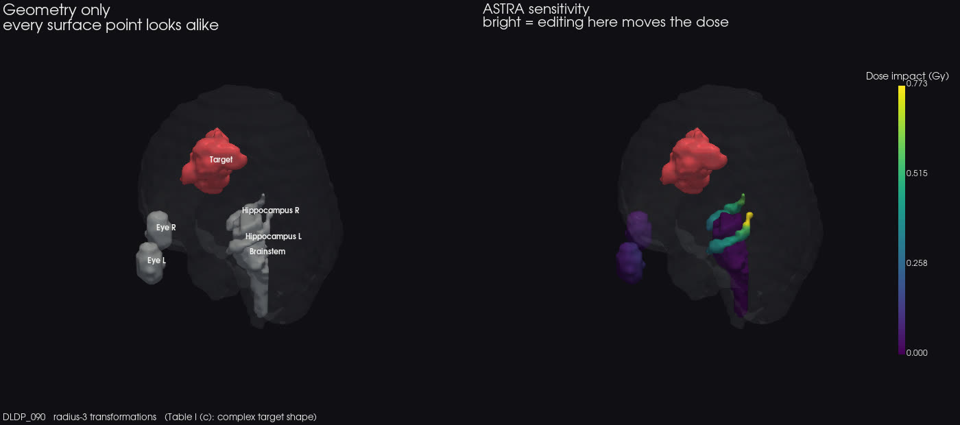
Each clip is a rotating 3-D rendering: a near-transparent brain for anatomical context, the target volume in red, and the organs at risk as surfaces, shown either uncoloured or coloured by the sensitivity map. The colour scale is in Gray and reports the mean absolute change in predicted dose over the brain.

The procedure, one perturbation at a timeFifty consecutive points along the brainstem surface. At each, the ball added to the contour is shown in yellow, the dose is re-predicted, and the resulting change is written onto the surface, so the map accumulates over the sequence.

A complex target shapeContours alone on the left, the sensitivity map on the right. The largest estimated dose change is at the edge of the left hippocampus, plausibly because it lies on critical beam angles.

A target close to the hippocampi and the brainstemIn this case the inferior parts of the eye show larger dose changes than the superior parts, which is the reverse of the other cases shown. The spatial pattern therefore depends on the individual plan rather than on the organ alone.

A small target, distant from the organs at riskThe smallest target of the twenty test cases, roughly 3 cm from the organs at risk. The points with the largest dose change are those nearest the target, and the overall scale is small, with a maximum of 0.17 Gy.

A larger targetThe dose change is distributed over more of each surface and the maximum rises to 0.61 Gy. The region of largest change on the brainstem lies away from the target rather than towards it.

Effect of the perturbation radiusThe same brainstem at perturbation radius 3, 5 and 7 voxels, each panel scaled to its own maximum. The magnitude of the dose change increases with radius while the spatial pattern is largely unchanged.

Results

Estimated dose change per organ at risk

Mean absolute change in predicted dose over the brain, in Gray, averaged over every transformation on that organ's surface. Four patients, in order of increasingly demanding target geometry.

Patient	Brainstem	Eye L	Eye R	Hippocampus L	Hippocampus R
small target, far away	0.007	0.012	0.009	0.104	0.082
larger target	0.016	0.049	0.059	0.374	0.271
complex target shape	0.010	0.042	0.029	0.309	0.263
target close to the organs	0.019	0.061	0.052	0.367	0.315

Down a column, the same organ differs by up to an order of magnitude between patients. Across a row, the hippocampi show 15 to 20 times the dose change of the brainstem in the same patient, despite the brainstem being roughly ten times larger and also close to the target. These values therefore depend on the individual plan and cannot be tabulated once per organ and reused.

Association with distance to the target volume

For each organ at risk, the Pearson correlation over its surface points between the dose change from a perturbation and the Euclidean distance from that point to the target volume. Averaged over the 10 test patients; organs ordered by mean size.

The three largest organs, the brainstem and both eyes, show negative correlations, strongest for the eyes: on a surface with a near and a far side relative to the target, points on the near side show larger dose changes. The smallest structures — cochleae, optic nerves and chiasm — are near zero, consistent with a structure only a few voxels across having little internal variation in distance. The left lacrimal gland shows a positive correlation, which is consistent with a structure lying outside the high-dose region, where dose is determined more by scatter and beam entry than by proximity to the target.

The values plotted here are recomputed from the archived volumes and differ in one row from those printed in the paper; see the errata.

Discussion

The maps can be computed before review. They are derived from the contours and the predictor alone, and indicate which surface regions would alter the predicted dose if redrawn. This is a more specific target for review effort than the contour as a whole.
Values do not generalise across patients. The same organ varies by up to a factor of 15 depending on target position, so a fixed per-organ ranking would be misleading in most cases.
Geometric overlap is a different quantity. Two contours differing in a low-sensitivity region produce similar dose; two differing in a high-sensitivity region do not, regardless of their overlap.
Limitation: the maps report dose difference, not constraint violation. Clinical decisions are made against dose constraints, and linking the two is the natural next step. A further limitation is that a separate predictor is required per tumour site, delivery machine and planning system.
Limitation: the perturbation model is isotropic. A ball added at a single point represents local over-segmentation only; under-segmentation and anisotropic disagreement are not covered here.
All reported values are recomputed from the archived volumes by the code in the repository, which also re-runs perturbations through the archived weights to check the stored maps against the model that produced them.

Errata

Every value on this page was recomputed from the archived planning volumes and sensitivity maps rather than copied from the paper. 66 of the 68 numbers the paper reports reproduce; the two that do not, and one methodological clarification, are listed below. The per-claim record is in results/embc_verification.csv in the repository.

Table II, right optic nerve

Quantity	Published	Corrected
Correlation with distance to target	−0.15	+0.25
Correlation with local dose gradient	+0.05	−0.11

Both signs are reversed. We could not recover the published pair from any subset of the twelve archived patients, nor under weighted or Fisher-z averaging; the closest any variant comes is 0.23. The remaining twelve organs reproduce to within 0.06. The corrected values place the right optic nerve alongside the left as a structure whose sensitivity is not explained by distance to the target, which does not change any conclusion drawn in the paper.

Table II, basis of the organ-size column

The paper describes an analysis over ten test patients. The published size column reproduces exactly — all thirteen values to within 0.01 voxels — as the mean over the first seven patients (DLDP_081 to DLDP_087) and not over any set of ten. The correlation columns behave the other way round, reproducing over ten patients and not over any subset of seven. The size column should therefore be read as a seven-patient mean; the correlations are unaffected. Sizes over all ten patients are, in the paper's row order: 2044, 44.3, 8.7, 8.6, 609, 601, 181, 195, 76.2, 76.7, 54.1, 57.4, 60.0 voxels.

Citation

@inproceedings{kamath2023astra,
  title        = {ASTRA: Atomic Surface Transformations for Radiotherapy quality Assurance},
  author       = {Kamath, Amith and Poel, Robert and Willmann, Jonas and Ermis, Ekin and Andratschke, Nicolaus and Reyes, Mauricio},
  booktitle    = {45th IEEE Engineering in Medicine and Biology Conference (EMBC)},
  year         = {2023},
  organization = {IEEE}
}